Results for Present-Day Conditions

Ramp-Up - FVCOM uses a mode-splitting technique in which the barotropic or external solution is computed at frequent intervals while the internal mode is computed at longer intervals.  For all our runs, the external time step was 0.55892 seconds while the internal time step was five times longer, or 2.7946 seconds.  80,000 external and 16,000 internal times steps equal one M2 tidal cycle.  The simulation is started from rest with the tidal forcing ramped using a cosh function with a time constant equal to 30,000 x 2.7946 sec, or ~23.3 hrs.  All the initial runs were run for 200,000 internal time steps or about 155 hrs.  The figure to the right shows the initial ramp-up and that steady tidal conditions were reached about a third of the way into the run.  The upper panel shows surface elevations at 4 locations just outside the inlets and 16 locations within the Bay.  The water elevation shown in the lower panel indicates the conditions at the end of the run the timing of which is indicated by the red dot in the upper panel.  The difference in the tidal excursions and the time lag between outside and inside the Bay is very clear.  Also clearly visible is the increase in mean water level by ~10 cm that develops inside the Bay with time.  This is due to the Stokes flow accompanying the progressive tidal wave into the Bay which is balanced by an outward Eularian pressure gradient.  For the purposes of determining the tidal-mean conditions discussed below, we have averaged over the last tidal cycle.

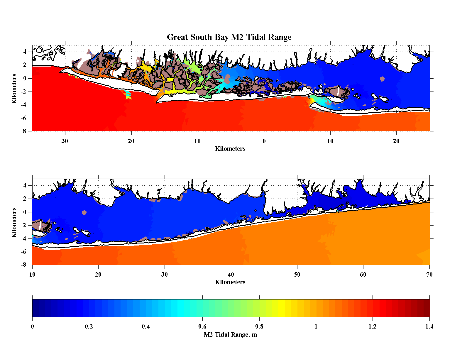
Tidal Range - Tidal amplitudes along the outer boundaries of the model domain range from a high of 0.68 m near Sandy Hook, to 0.48 m off Montauk.  This results in tidal ranges at those two extremes of 1.36 m and 0.96 m, respectively.  Inside the Bay the tides are much attenuated and there is a substantial phase lag between high tide at the inlets and that along the north shore.  The model predicts a phase lag between Fire Island and Bellport Bay of ~3.9 hrs as compared to the tide tables which indicate a lag of 3.8 hrs.  The tidal range, the difference between high and low tides, in Great South Bay is about 0.3 m over most of the bay, slightly less in Moriches Bay and significantly higher in the western Bay.  The reduced attenuation in the western Bay is attributed to the relatively small volume of water in that area with its extensive tidl flats and narrow channels.

 

Temperature and Salinity - The upper figure at the right shows the evolution of the temperature and salinity in the Bay during and after the ramp-up period.  We are not forcing the model with surface heat fluxes so the temperature is not particularly realistic.  Salinity however is being realistically forced through internal exchange within the Bay, fresh water forcing from the rivers, submarine ground-water discharge and exchange through the inlets.  Given the approximate nature of the initial conditions and fresh water fluxes, there is surprisingly little salinity adjustment needed in the sumilation.  There is almost no change in Bellport Bay (node 55367) or the middle of the Bay south of Sayville (node 48493).  Only node 14775 east of Jones Inlet indicates any real adjustment.  Otherwise the dominant variability is that associated with the tidal fluctuations.  The lower panel shows the depth-averaged temperature and salinity within the Bay at the end of the run.  As the figure in the ramp-up discussion shows, the end of the run coincided with a falling tide through most of the Bay and low tide on the shelf and inlets.  (The dots in the figure show the positions of the nodal temperatures and salinities shown in the upper panel.)  In terms of salinity, the figure gives a good overview of the salinity distribution with the highest salinities in Moriches Bay, intermediate to high salinities in the western Bay and lowest salinity in Patchogue and Bellport Bays.

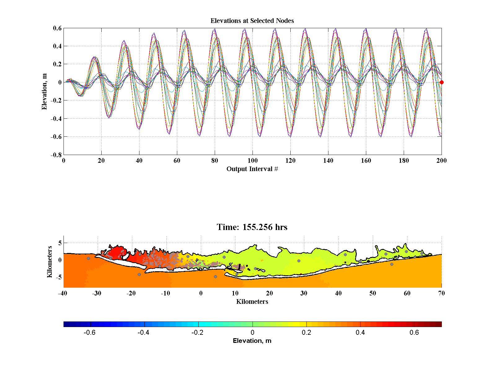
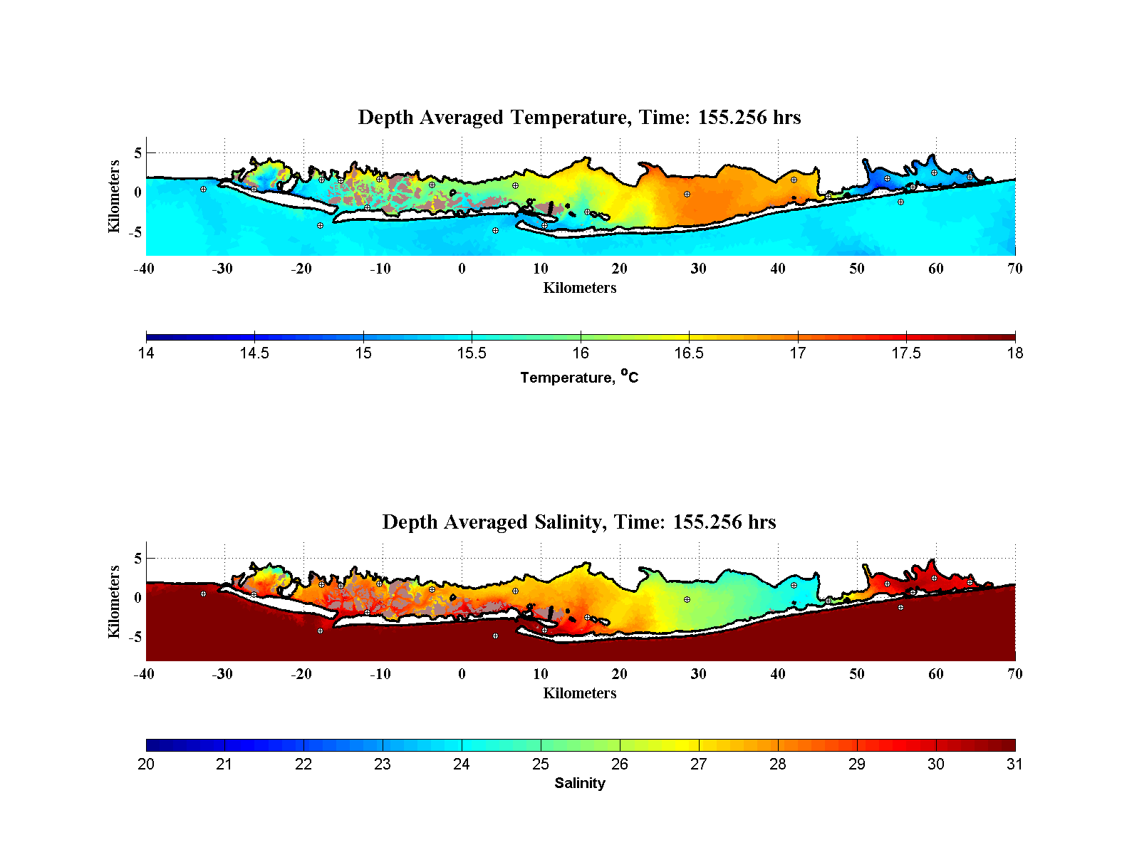
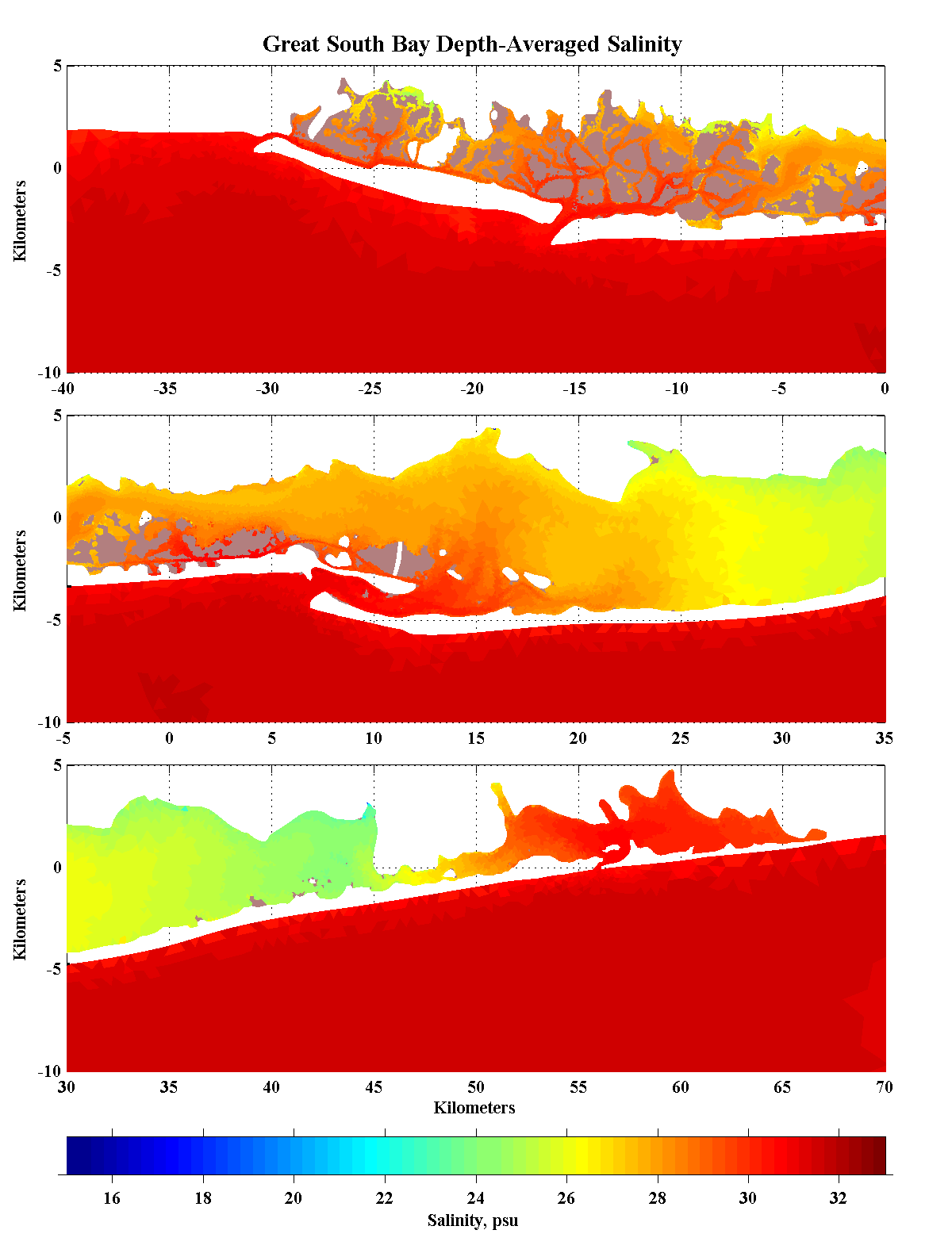
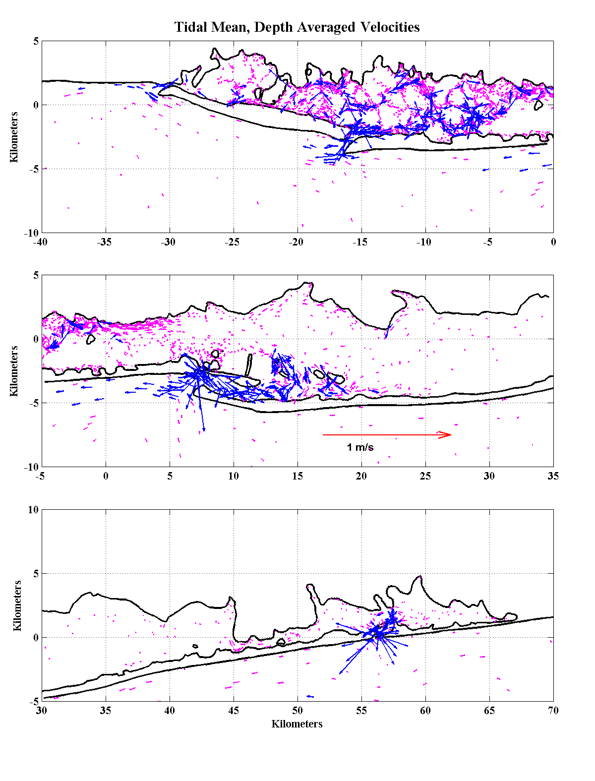
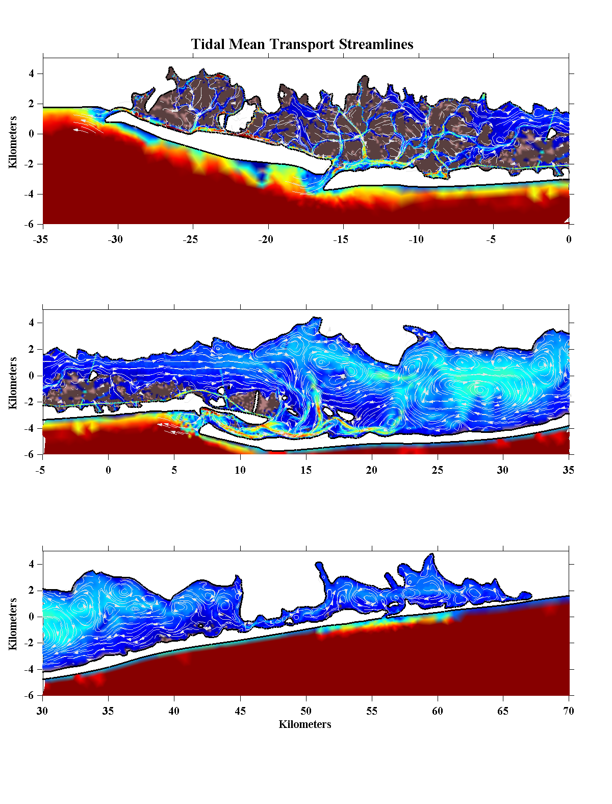
Base-Case, Tidal-Mean Conditions -    The panels below show tidal-mean conditions from the last 12.4 hours of the ramp-up discussed earlier.  In terms of tidal currents and elevation the simulation appears to have reach equilibrium while salinity appears close to equilibrium except in some of areas remote from the inlets and where our initial conditions were poorly constrained by observations.     The first panel shows the tidal-mean elevation where the overall set-up within the Bay is clear.  The set-up is both the highest and lowest in the western reaches.  As mentioned earlier, the setup is caused by the Stokes drift accompanying the incoming tide and is largest where the tidal flow is constricted.  As a result the largest set-up occurs along the north shore of the Bay to west where access to the ocean tide is restricted by the many narrow and shallow channels.  The southern portion of this same area shows some of the lowest set-ups and this seems to be caused by the proximity of East Rockaway and Jones Inlets and the relatively small volume of water in this shallow end of the Bay.  Over the rest of the Bay and into Moriches Bay, the set-up appears to be about 8 cm, a little higher in Smith Point Channel and there is a clear setup minimum in the proximity of Fire Island Inlet which is responsible for the net outflow through the Inlet.     The top right -panel shows the tidal- and depth-averaged salinity.  As mentioned above, the highest salinities are in Moriches Bay, the Area in and north of Fire Island Inlet and in the shallows channels of the western Bay.   The lowest salinities are found in Bellport Bay and at locations along the north shore where freshwater enters the Bay from rivers and creeks.  For a point of reference, we have a long-term salinity record from the north shore of Bellport Bay (see the section on monitoring results) where the mean salinity is about 24 psu and is very close to what the model simulation shows.  We have a shorter record from Tanner Park (located on the north shore at 2km) which shows much more variability with a rough estimate of mean salinity of around 27.5 psu.  In that area the simulation shows a pool of relatively low salinity water of around 26 psu.  However in the simulation, areas east and west of Tanner Park show an increasing salinity with time to values of 28 psu so it appears that the model has not quite reached equilibrium at this location which is well removed from inlets.    The bottom panels show the tidal- and depth-averaged velocities and the tidal-mean transports.  In the left panel the magenta vectors show currents between 1 and 5 cm/sec while the blue vectors shows currents between 5 and 50 cm/sec.  The vector plot has been heavily decimated while velocities less than 1 cm/sec are not shown.  Examination of the mean currents shows that the largest residual currents occur in the inlets, in the channels and along the north shore of the western Bay and in Smith Point Channel.  The residual currents are much smaller in the open central Bay area.  An important point brought out by this figure is that, generally, there is a mean inflow in three smaller inlets, East Rockaway, Jones and Moriches, and an outflow through Fire Island Inlet.  Thus, both the western and eastern ends of the Bay are supplying more saline waters to the central Bay to maintain the salinity balance against the influence of the larger rivers.  Greater detail about the interior flow pattern is shown by the transport streamlines which  indicates the presence of a number residual eddies in the open portions of the Bay.  Most of the headlands seem to have an associated eddy and there is a large clockwise eddy south of Sayville.  An important feature illustrated in the streamlines is the eastward flow out of Great South Bay south of Lindenhurst and Babylon supplying a major portion of the outflow through Fire Island Inlet (see below).

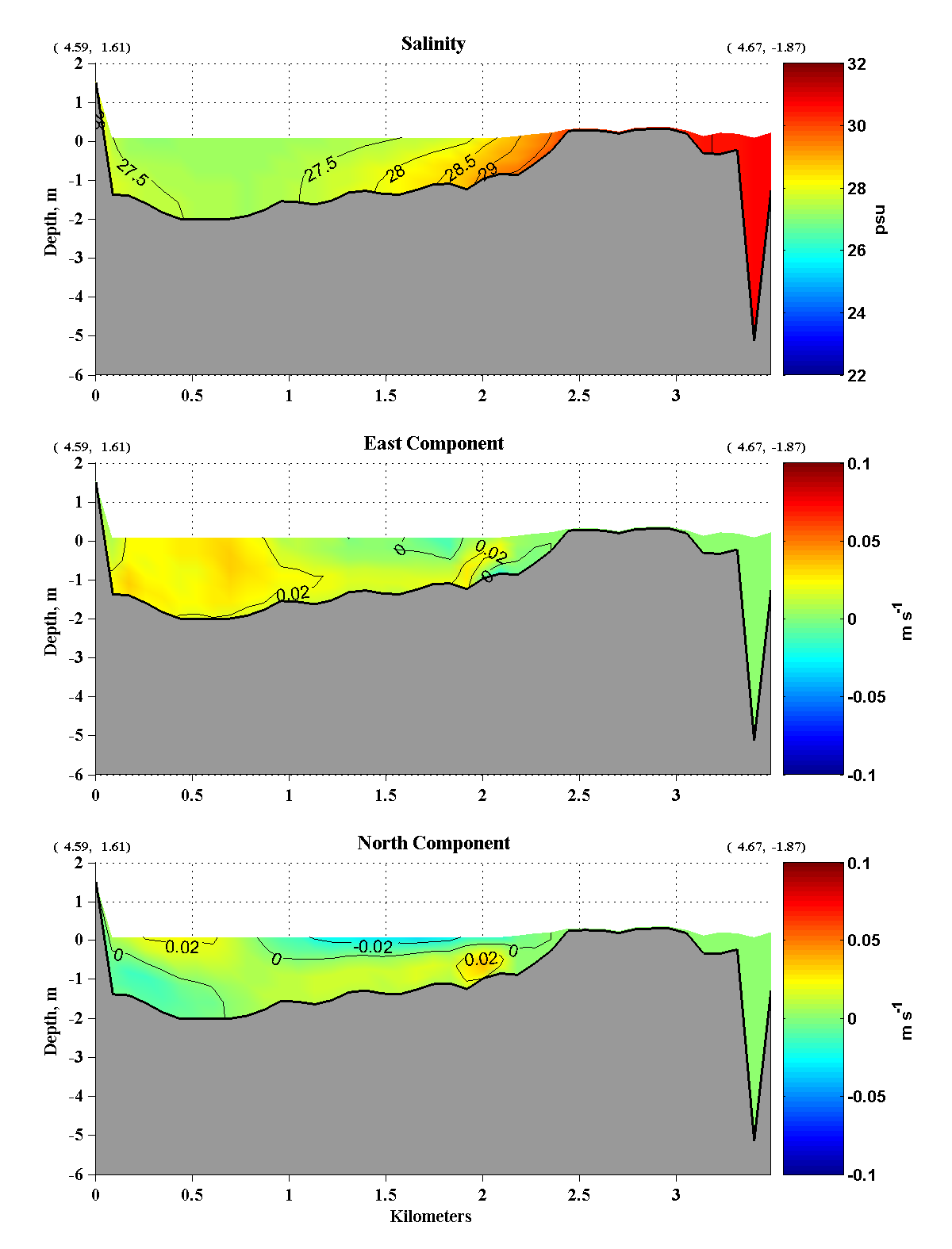
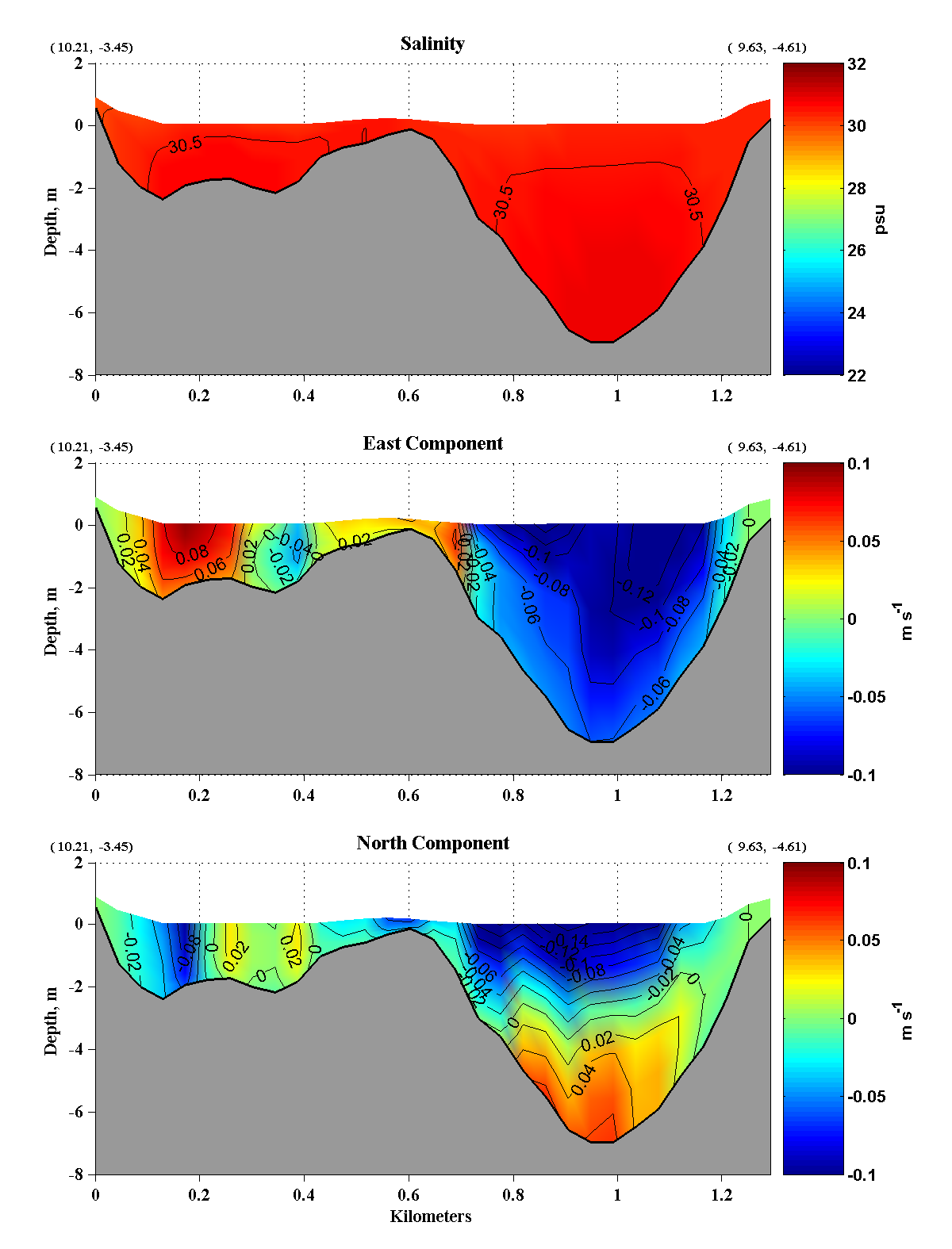
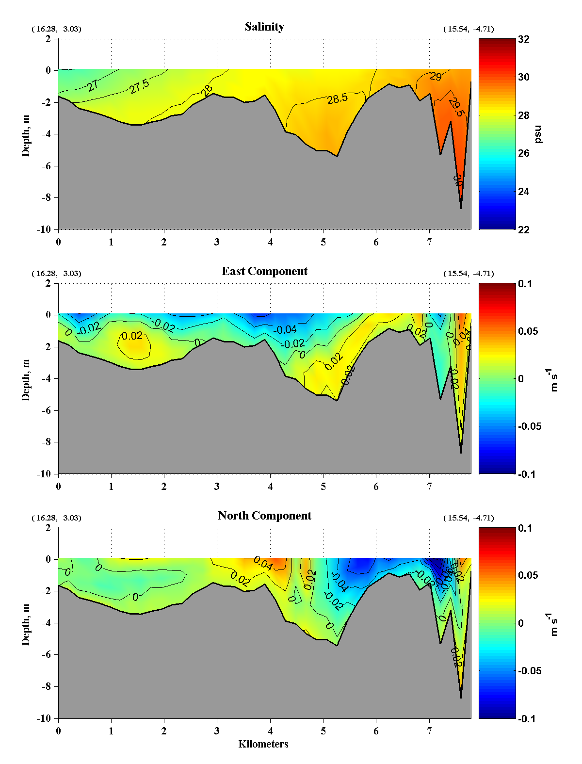
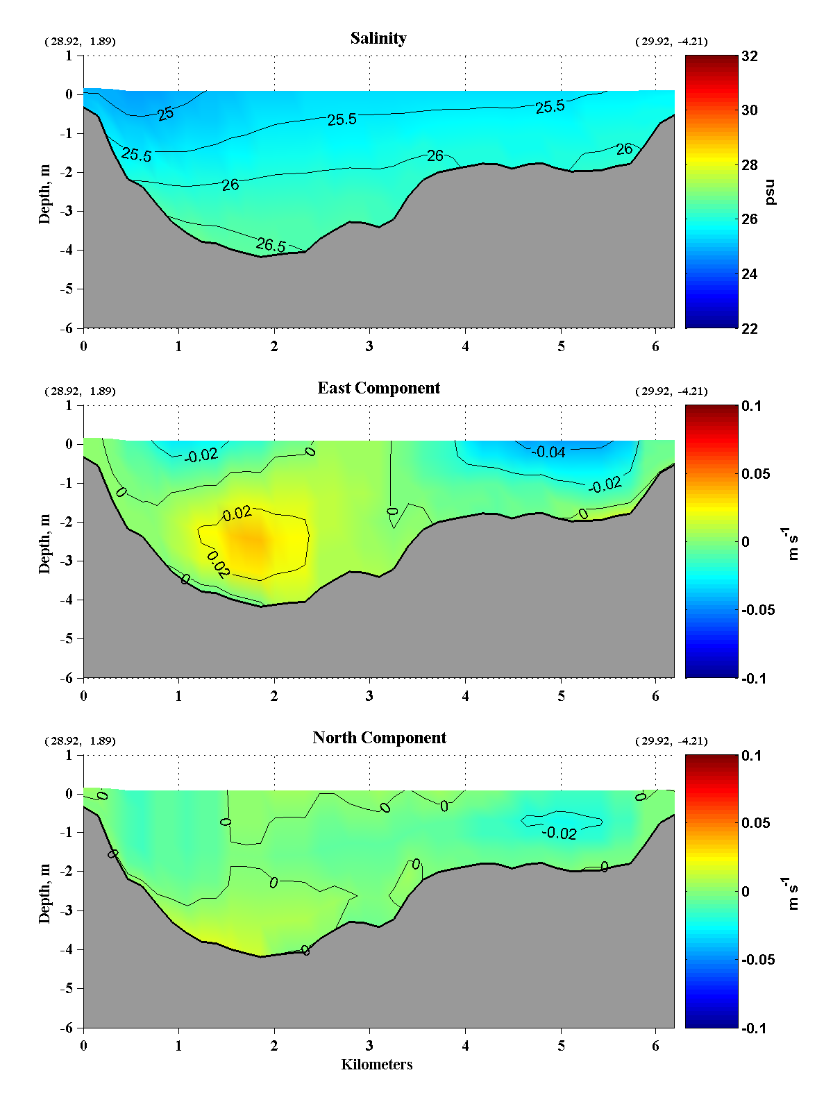
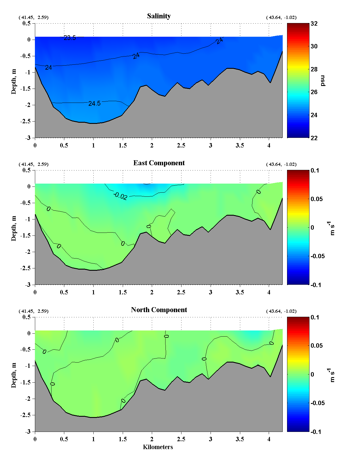
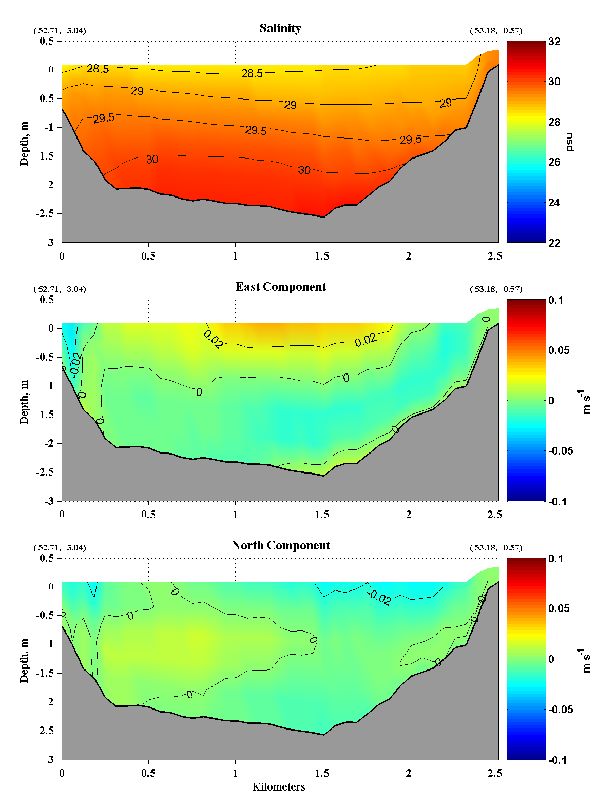
Vertical Sections A series of sections have been generated to show the vertical and horizontal structure of the salintity and velocities under the base-case conditions.  The chart below shows the locations of the vertical sections while the lower panels show vertical sections of the tidally-averaged salinity and nominally, east and north velocity components.  (The velocity components have been rotated 15o  to be aligned along and across the Bay so that the "east" component is actually toward 75oT while the "north" component is toward 345oT.)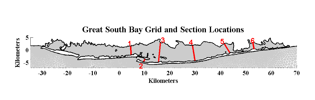 (1) (2) (3) (4) (5) (6) In looking at these figures it is important to remember that the circulation and salinity distributions were computed without any wind stress or radiative forcing so that a somewhat greater than normal degree of stratification is evident.  The advantage of this presentation, however, is that it shows the tendencies of the horizontal and vertical density distributions. Thus, the estuarine nature of the circulation is clear with more saline waters laying along the bottom and fresher surface waters which are found predominantly along the north shore.  However, the circulation is not a simple reflection of the salinity distribution.  In the central and eastern portions of the Bay (sections 3, 4 and 5) the deeper saline waters are moving eastward into the back Bay areas while there is a tendency for the near surface layers to move westward but this is not limited simply to the lowest salinities in each section.  In western half of Moriches Bay higher salinity waters flow westward along the bottom while lower salinity waters flow eastward.  The flow in Fire Island Inlet shown in the second panel consists of water of higher salinity than that found in the Bay but lower than that offshore.  Thus, the mean westward outflow of water through the main channel is carrying fresh water out of the Bay to maintain the salinity balance against the influences of the rivers and bottom fresh water supply.   The north-south velocity gradient in the inlet highlights one of the difficulties in illustrating the mean tidal flow.  Because of the channel curvature up and downstream on the section, outflow during ebb-tide preferentially follows the south channel while there is a greater impact of the flood tide in the north channel.