
University of Rhode Island
| |
University of Rhode Island |
| The Norrona Project |  |
| Charles N. Flagg
E-mail: Charles.Flagg@sunysb.edu School of Marine and Atmospheric Sciences Stony Brook University Stony Brook, NY 11794 |
H. Thomas Rossby
E-mail: trossby@gso.uri.edu Sandy Fontana E-mail: sfontana@gso.uri.edu Graduate School of Occeanography University of Rhode Island Narragansett, RI 02882 |
ADCP Data Retrieval XBT Data Retrieval TSG Data Retrieval |
|
The
MV Norrona is a large, high-speed ferry, based in Torshavn
on the Faroes Islands and operated by the Faroese company,
Smyril Lines p/f.
that makes weekly runs between Denmark and Iceland.
This route crosses the northern limb of the Meriodional
Overturning Circulation and thus, appropriately
instrumented, the ship affords an opportunity to monitor
one of the most important components of the world climate
system. The Norrona Project is a joint effort by
Stony Brook University and the University of Rhode Island,
funded by the National Science Foundation, to equip the
Norrona with an Acoustic Doppler Current Profiler (ADCP)
to begin a long-term monitoring of the northward flow of
the warm North Atlantic waters through the Faroes-Shetland
Channel and over the Faroes-Iceland ridge into the
Greenland and Norwegian Seas. European collaborators
have recently joined the effort and have established a
"Ferry Box" system on the Norrona to record near-surface
temperature and salinity. This web-site describes
the program goals, the installation of the ADCP system on
the Norrona, the efforts to over-come significant bubble
sweep-down effects, and provides access to the data as it
becomes available. Introduction Background The ADCP System and Installation Bubble Sweep-Down Bubble Fairing Results and Data Pictures Acknowledgements: This project has been possible only through the extraordinary help and collaboration from Smyril Lines, especially that of Captain Jogvan Davastovu, the captains, engineers and electronics officers of the ship, and shoreside network administrators. The work has been funded under a grant from the U.S. National Science Foundation. |
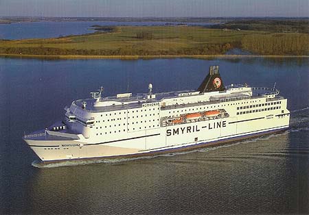 Smyril Line's high speed ferry Norrona (163.34 m x 30 m x 6 m) 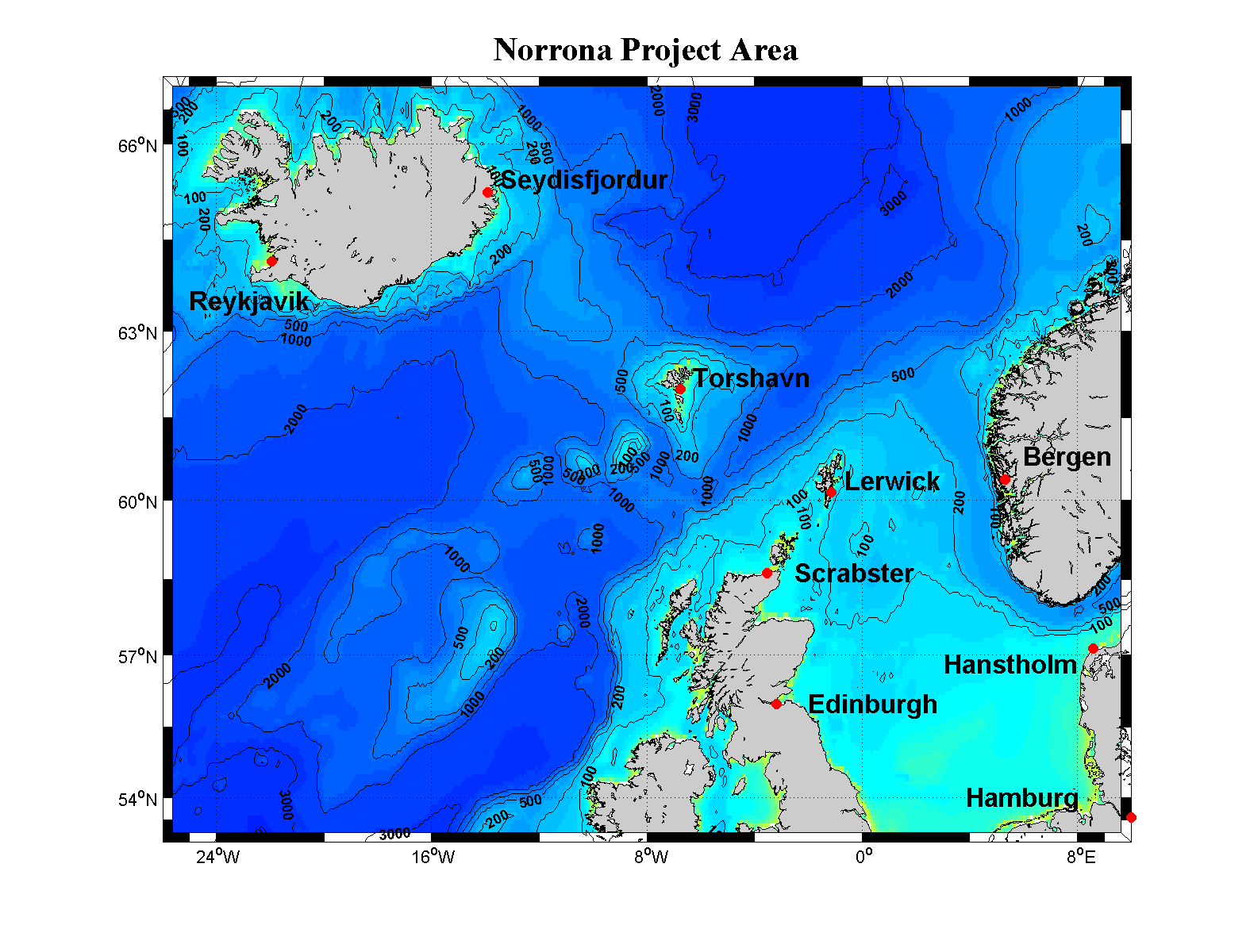 |
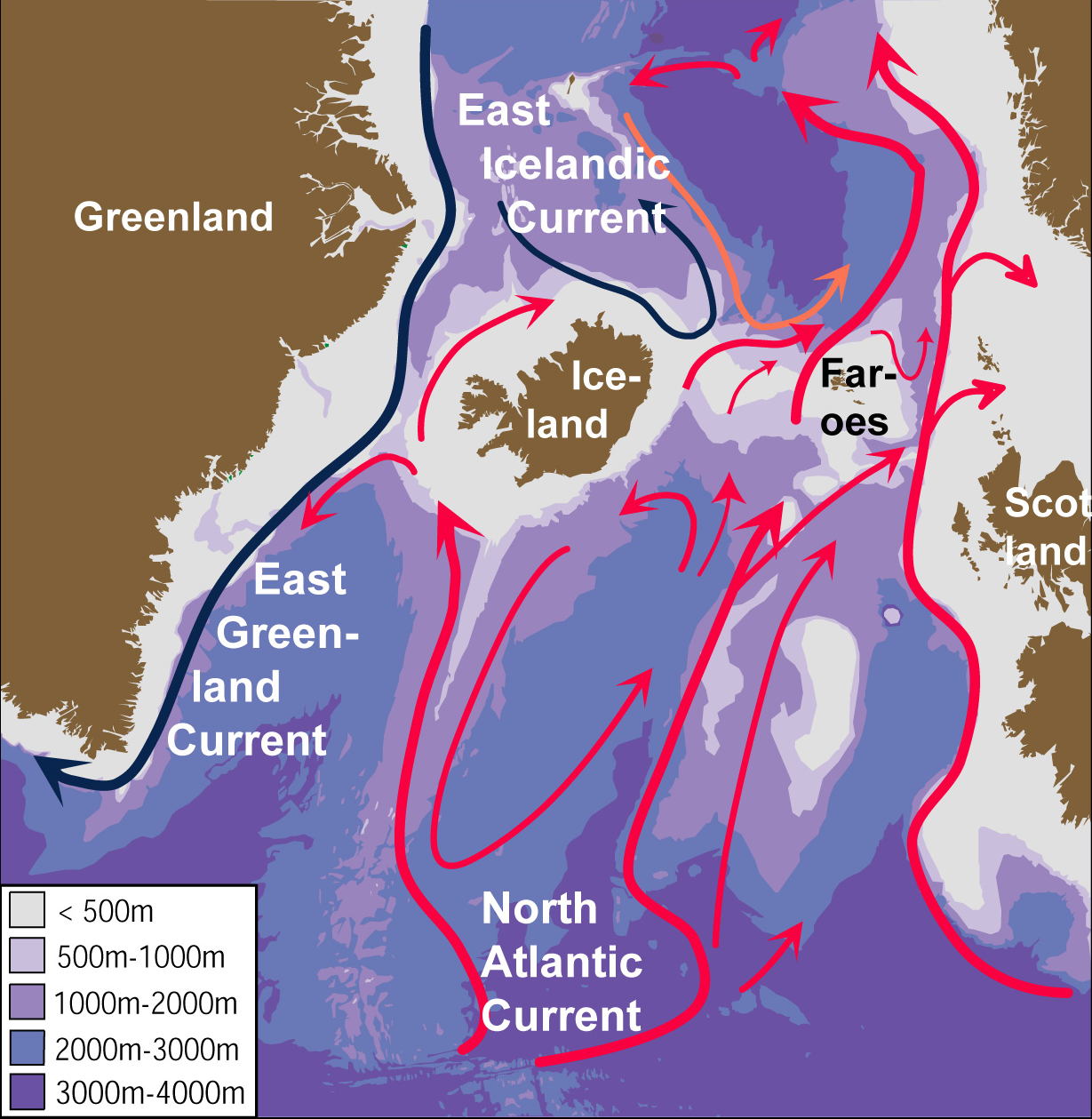
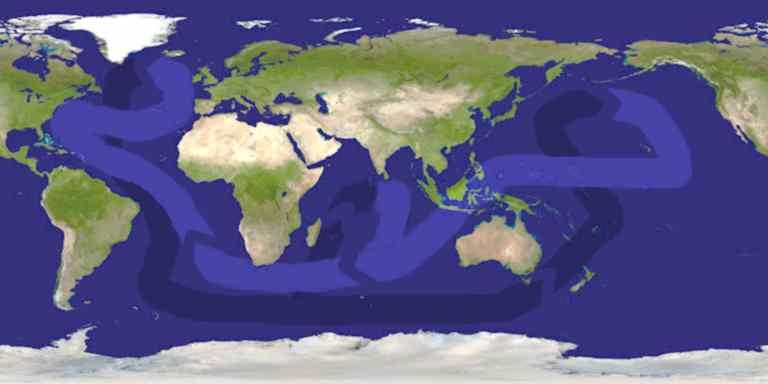
| Introduction The warm waters flowing from the Atlantic into the Nordic Seas past the Faroes play the primary role in moderating the climate of northern and central Europe. This flow, popularly known as the Gulf Stream, is such a natural part of our lives that we take it for granted. It forms the northernmost link of a global circulation that goes under names such as the global thermohaline circulation (THC), the meridional overturning circulation (MOC), but perhaps the most widely known term is the global conveyor belt, illustrated by the system of dark and light lines in the figure below. These warm and salty waters from the North Atlantic sink in the Norwegian Sea and spill back into |
the deep Atlantic and from there spread out into the global ocean (the dark blue band). They gradually warm, rise and flow back towards the North Atlantic (light blue line). Significantly, all the waters in this global circulation system flow past the Faroes even if the figure is too simplified to indicate this. Of central importance to this circulation as we know it, is that the waters sink and flow back into the deep North Atlantic. If they did not do so, there would be no demand for waters to replace this loss, and the inflow would decrease or stop (as it did during the last glacial period some 20,000 years ago). |
 |
|
| In recent years, as our information of the ocean and its variability has improved, we have learned that the flow varies considerably, and may be quite sensitive to changes in weather and climate. It is already known that the Shetland Current varies in response to winds over the northeast Atlantic. Recent research has indicated that as a consequence of global warming climate at high latitudes including the Nordic countries could actually become cooler. The reason for this is curious. Under present conditions the warm waters flowing north are salty, enabling them to sink to great | depths when cooled off in the high latitude winter. These dense waters then flow or spill back out into the deep North Atlantic and the global ocean. But if increased rainfall and ice melt freshens these waters, they may not become dense enough to sink in which case the demand for more warm water will cease - leading to a cooler perhaps even a cold climate at high latitudes. Thus, in these days of global warming there is much interest in monitoring the strength and salinity of this flow past the Faroes. The vessel Norröna provides an excellent platform from which to do this. |
| Recent
Research A number of research programs have been measuring currents in the Denmark Straits between Greenland and Iceland and along the ridge between Iceland, the Faroes and Scotland. The classic measurement technique is the moored (or anchored) recording current meter that measures the flow of water past the mooring and records the results internally. Such instruments have been deployed across the Faroe Bank Channel, located between the Faroes and Faroe Bank to the south to measure the outflow of cold water from the Nordic Seas back into the Atlantic. (This 800 m deep channel is the deepest connection between the Atlantic and Nordic Seas.) Similar instruments have been deployed across the Shetland Channel to measure the inflow of warm waters into the Norwegian Sea, and north of the Faroes to measure the volume of water transported by Faroe Current. These programs have greatly improved our knowledge of the exchange rates and how they vary with time, from season to season and from year to year. To date, the best estimate of inflow between Iceland the Faroes is 3.8 x 10⁶ m3/sec and just about the same amount in the Shetland Channel. For comparison, the outflows from all the rivers of the world sum to about 1 x 10⁶ m3/sec. The Norrona Project: The Norrona measurement program takes a different approach: It will measure currents from the surface to depths as great as ~800 m depth all along along the ship's track. Thanks to the twice weekly transits between Denmark and Iceland, throughout the year, year after year, the inflow and how it varies in time along the ridge |
can
be determined with unprecedented accuracy. Unlike
moored current meters, the Norrona will provide
substantially improved spatial coverage. Why does
this matter? We know that the inflow of water through the Shetland Channel varies depending upon winds over the northeast Atlantic. We also know that a decrease in transport cannot persist without causing the inflow to increase elsewhere (or the outflow to decrease) for otherwise the sea level in the Nordic Seas would likely begin to drop. By measuring currents throughout the region, we can begin to understand in detail how changes in one place lead to variations in another. Because the Norrona can measure currents to ~800 m it will also be able to measure the flow from the Nordic Seas back into the Atlantic. At depths below the 800 m (the sill depth of the Faroe Bank Channel) there should be little net flow south through the Shetland Channel. At shallower depths the Norrona will be able to measure any waters going south and eventually spilling into the deep north Atlantic. Thus the Norrona will be able to measure flows in and out and how they vary spatially and in relation to each other. But the most important question the Norrona program seeks to address is the long-term stability of the flow into the Nordic Seas of warm salty water, the upper branch of the global meridional ocean circulation. Some observations have indicated a possible weakening of the MOC, but the measurement uncertainties are huge. The complete coverage of the inflow provided by the Norrona will allow oceanographers to determine with significantly improved accuracy the inflow and how it varies in time and along the ridge. One might say that the Norrona will provide an early warming system for any change in this inflow and thus change in European climate. |
|
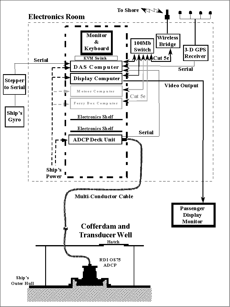
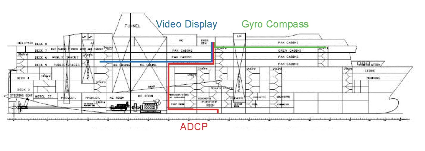
Cabling for the Norrona
ADCP System
 |
| Norröna's bulbous bow and bow thrusters  |
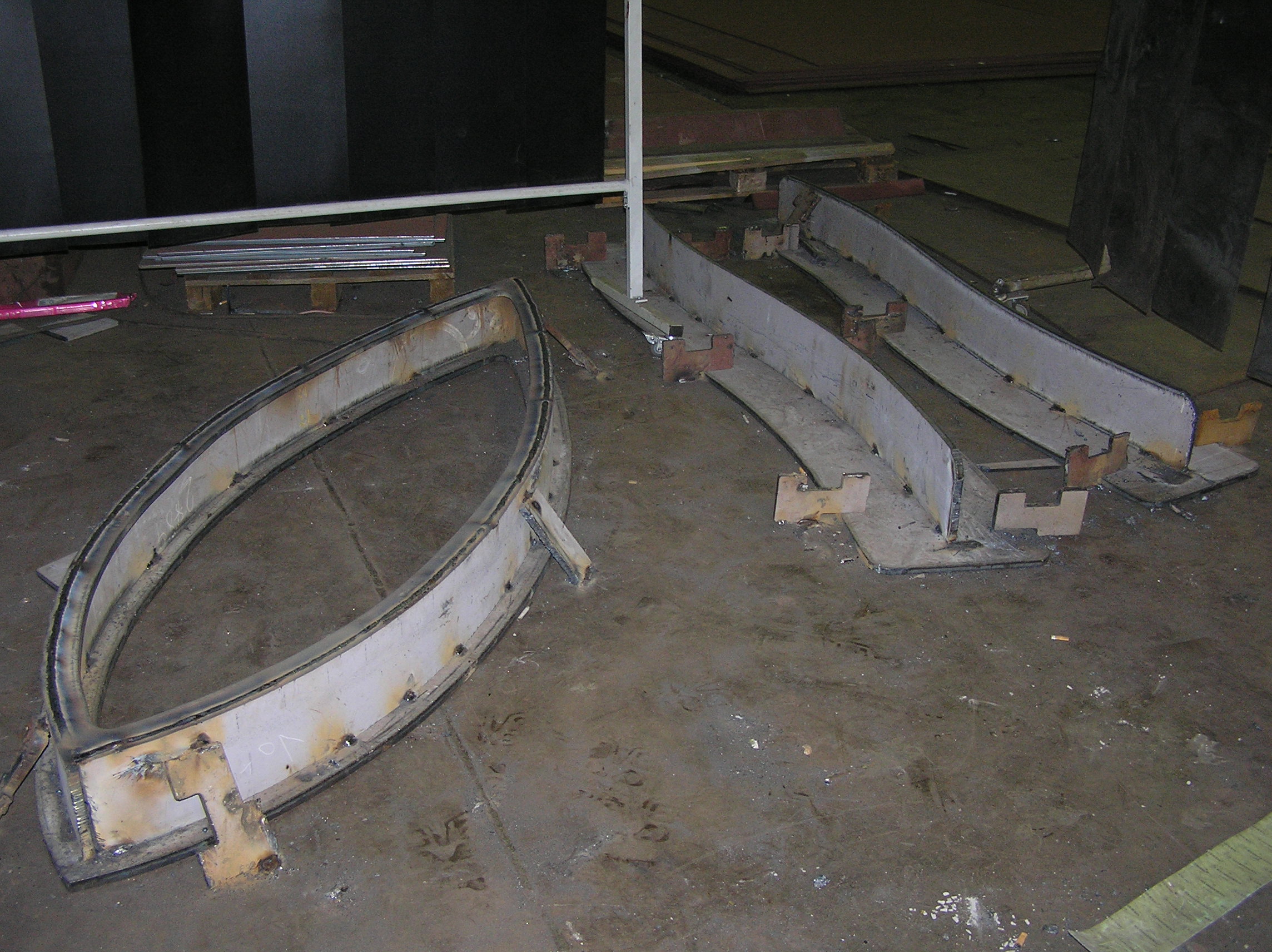
Temporary
bubble fairing |
Temporary
bubble fairing |
Temporary
bubble fairing |
% Good
with temporary fairing |
1st
permanent bubble fairing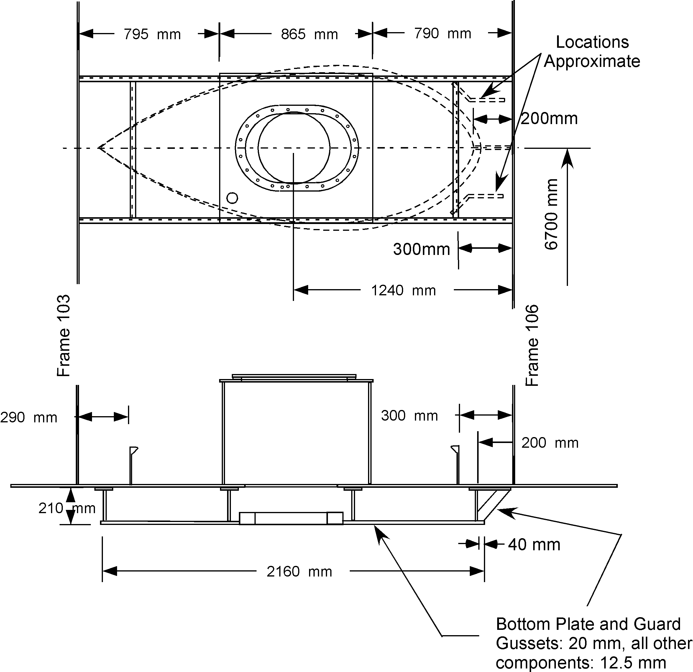 |
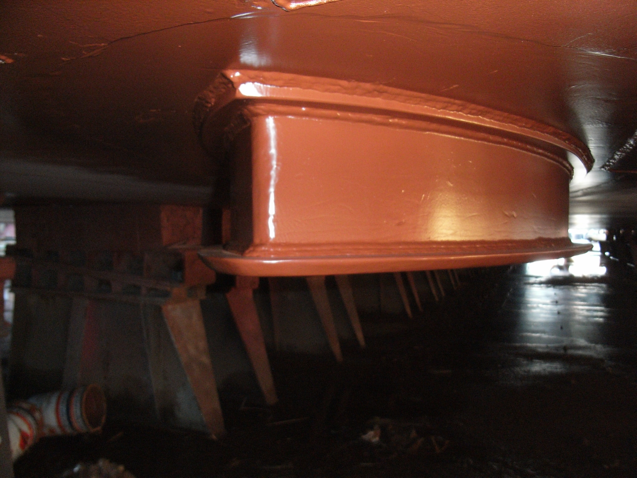
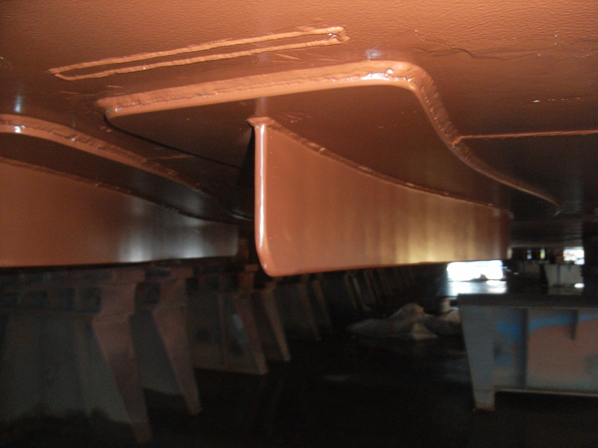
Permanent
bubble fairing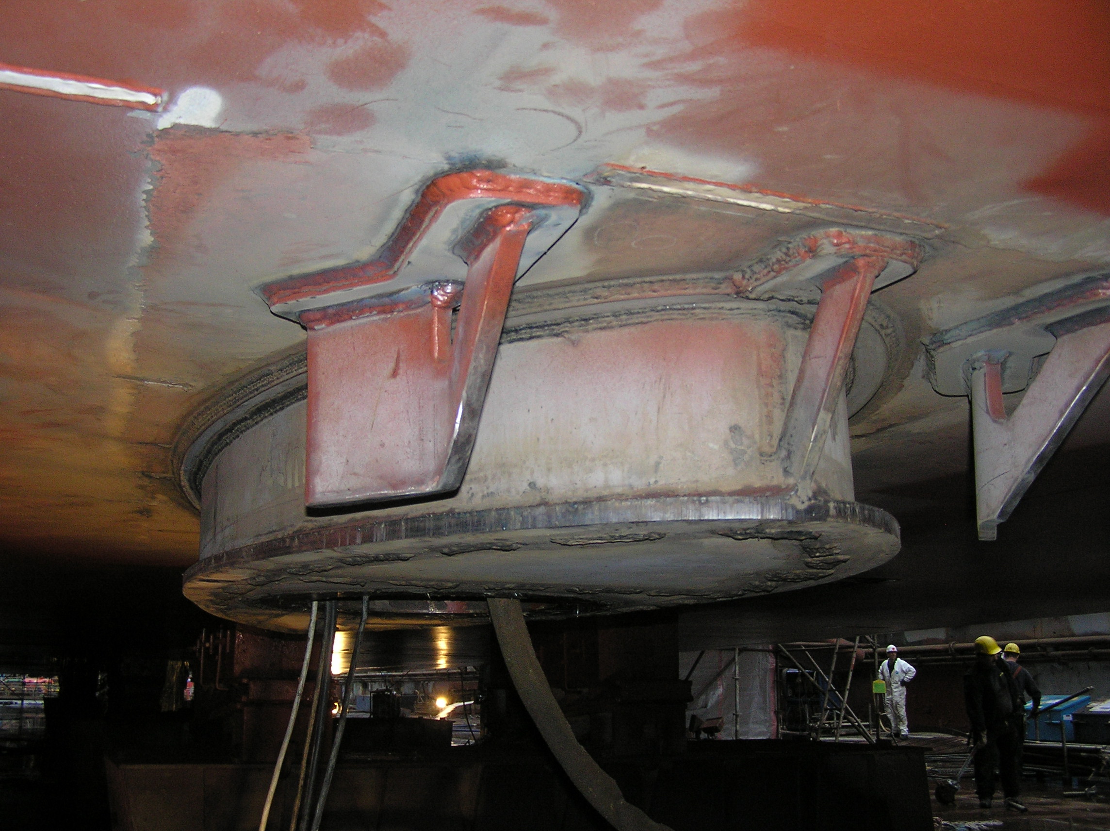 |
Modified
bubble fairing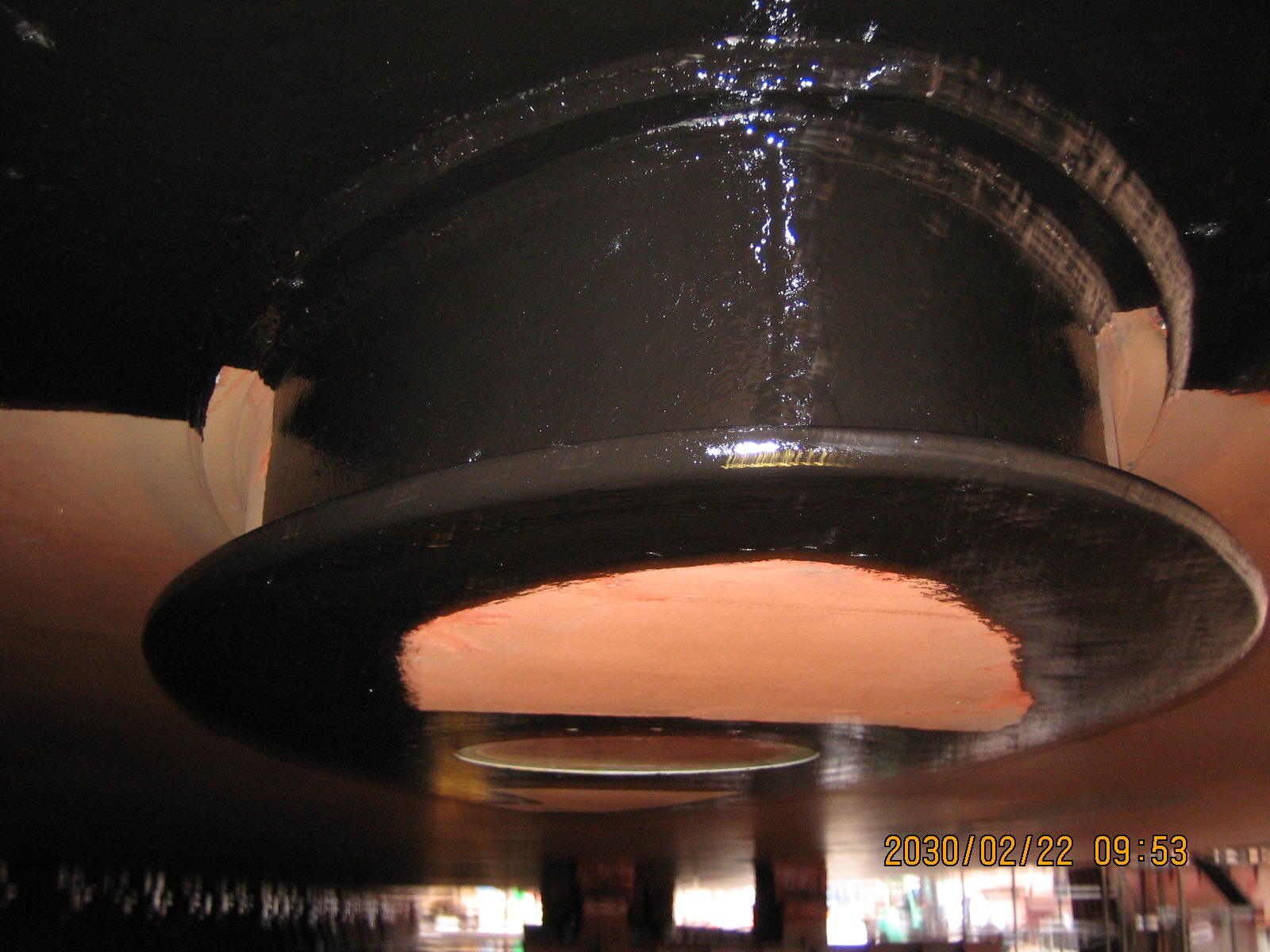 |
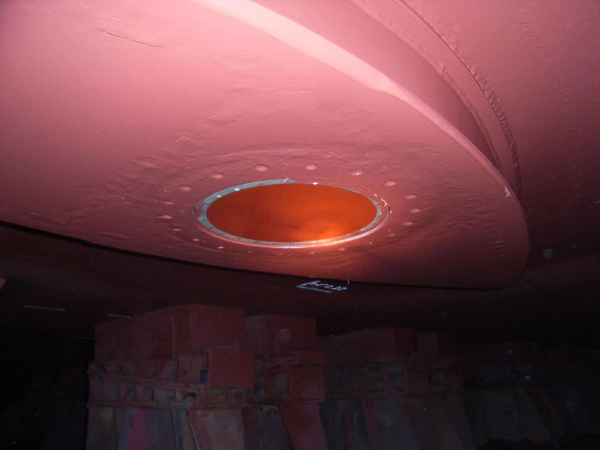
The updated version of the thru-hull
bubble sonar operates at 200 kHz as before but with an improved
digitization rate of 24 kHz, decimated to a sample rate of 240
Hz, yielding a vertical resolution under the hull of 3 mm. The operating frequency is determined
by the acoustic impedance of the 12.5 mm thick steel hull such
that the hull is nearly acoustically transparent and there is
maximum signal penetrating into the water.
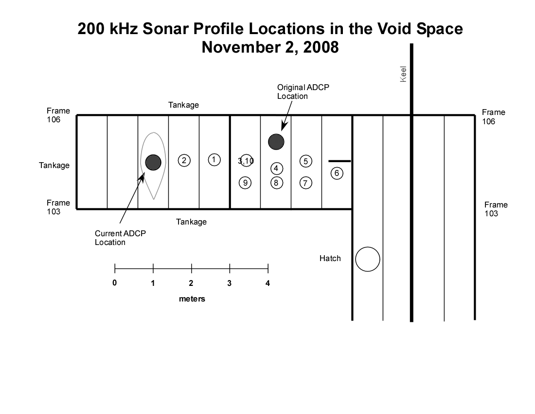
The transducer was moved to 18 places in the void space
where the ADCP could be located to see if there was an optimal
location. At each location 100
profiles were obtained over a period of one minute returning 120
backscatter estimates between 104 and 600 μsec
after the ping. The results that
were obtained by the sonar (see below) indicated high
backscatter close to the hull that decayed to background at
between 10 and 20 cm. The
background values corresponded closely with those obtained when
the ship was still at the dock. Occasionally,
we got high backscatter from a few pings farther from the hull
with the farthest high backscatter return from about 40 cm. The weather during the sonar runs was
fairly benign by
 |
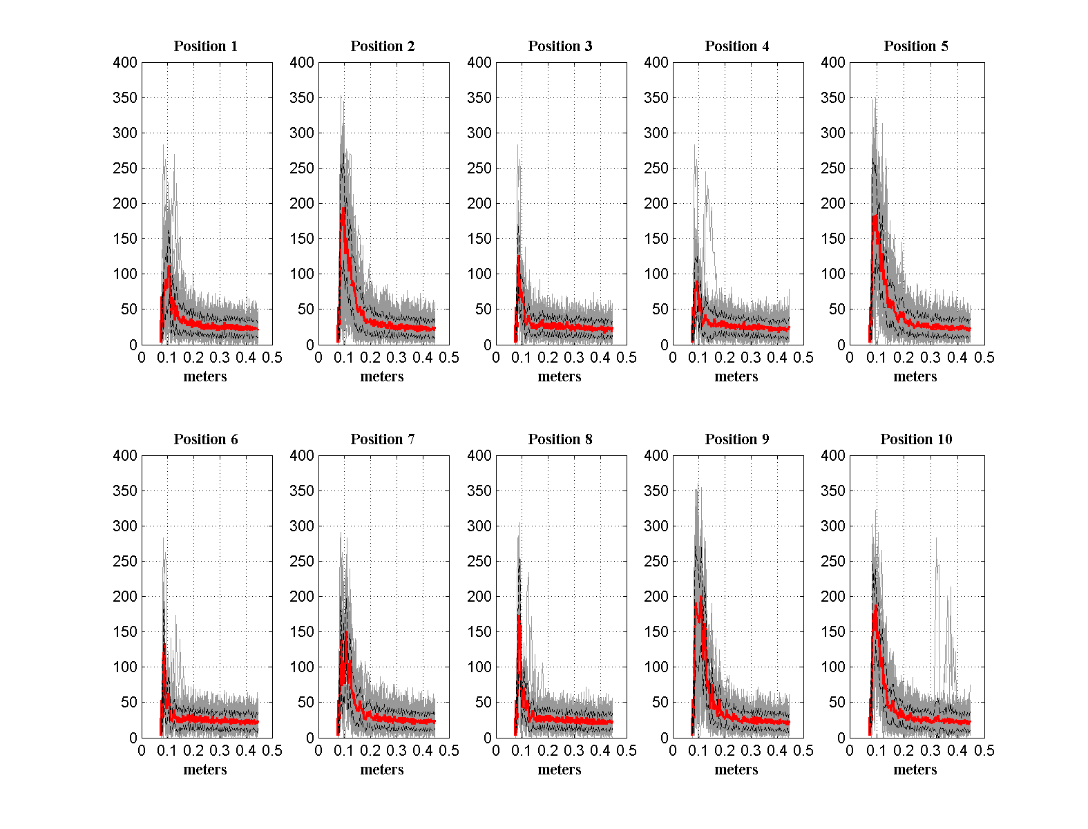 |
Results
from
the bubble sonar showing 100 backscatter profiles at a number
of locations as a function of distance below the hull.
The
underwater
camera was an attempt to get unequivocal evidence about the
character of the bubbles under the hull. The difficulty
with this approach was to find a camera that could operate
autonomously, record the pictures internally and be diver
deployable. It turns out that we were not the first with
requirements for an autonomous underwater video camera.
Greg Marshall’s group at the
National Geographic Society have been
developing their Crittercam for several
years so that they could attach it to various sea animals and
record their behavior. The latest version of the Crittercam is remarkably compact and can
record up to eight hours of video (and audio) data on internal
solid state memory.
| Streamline fiberglass shell,
and Crittercam on magnetic clamp 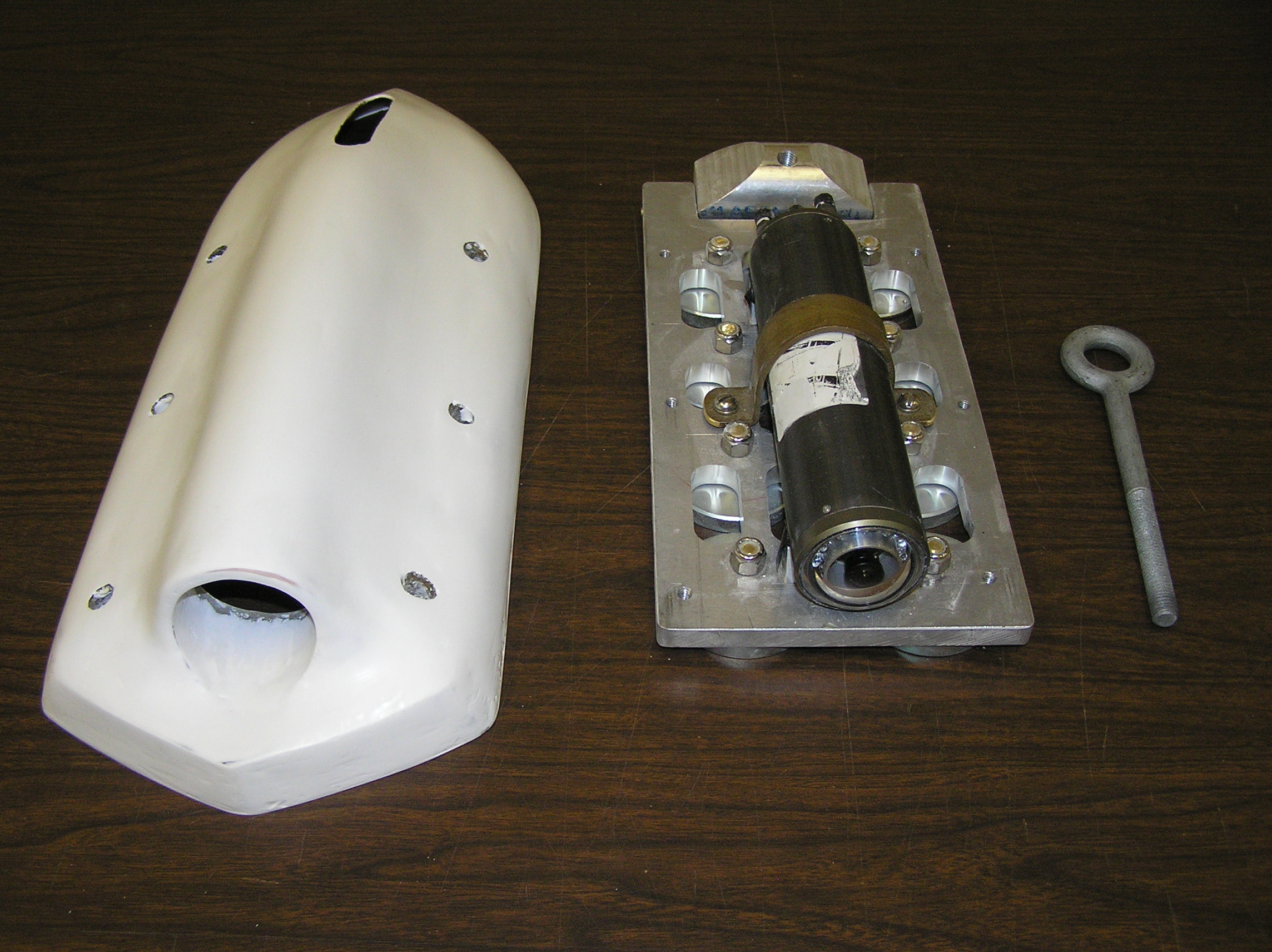 |
Assembled underwater camera system 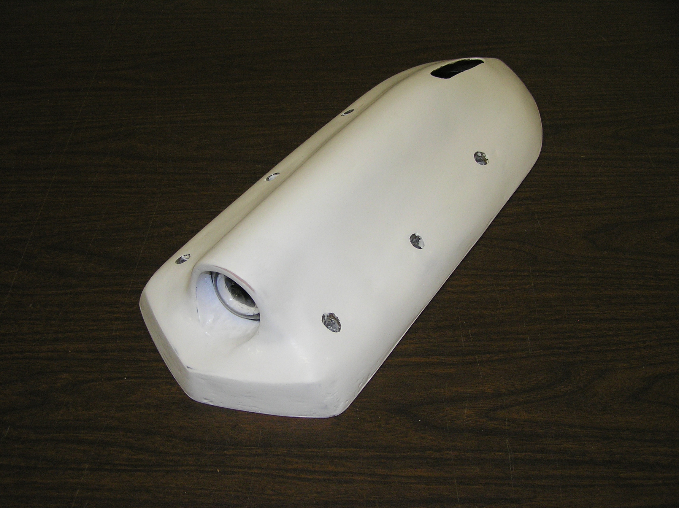 |
Camera positions under void space 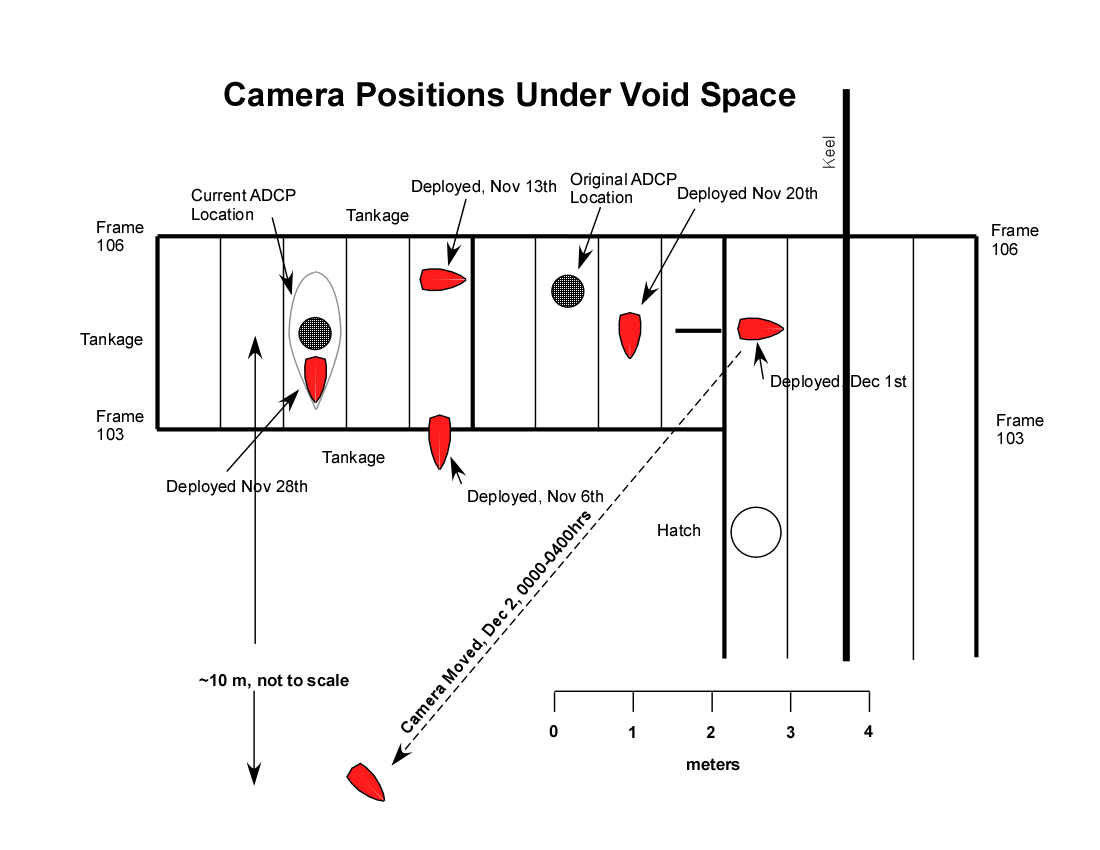 |
The camera was deployed at five
different locations with the help of Ebba Mortensen of the
Faroese Fisheries Institute and Edvard Kjeld a professional
diver operating in the Faores, to study the character of the
bubble clouds and to get some idea of their spatial
distribution. That there are
bubbles under the ship is indisputable from the camera results
and they are clearly the cause of the poor data return from the
ADCP. The most informative results
came from the videos taken during daylight hours when light from
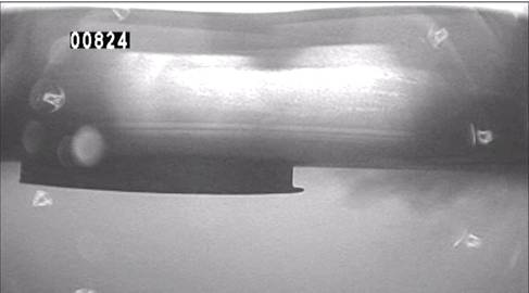
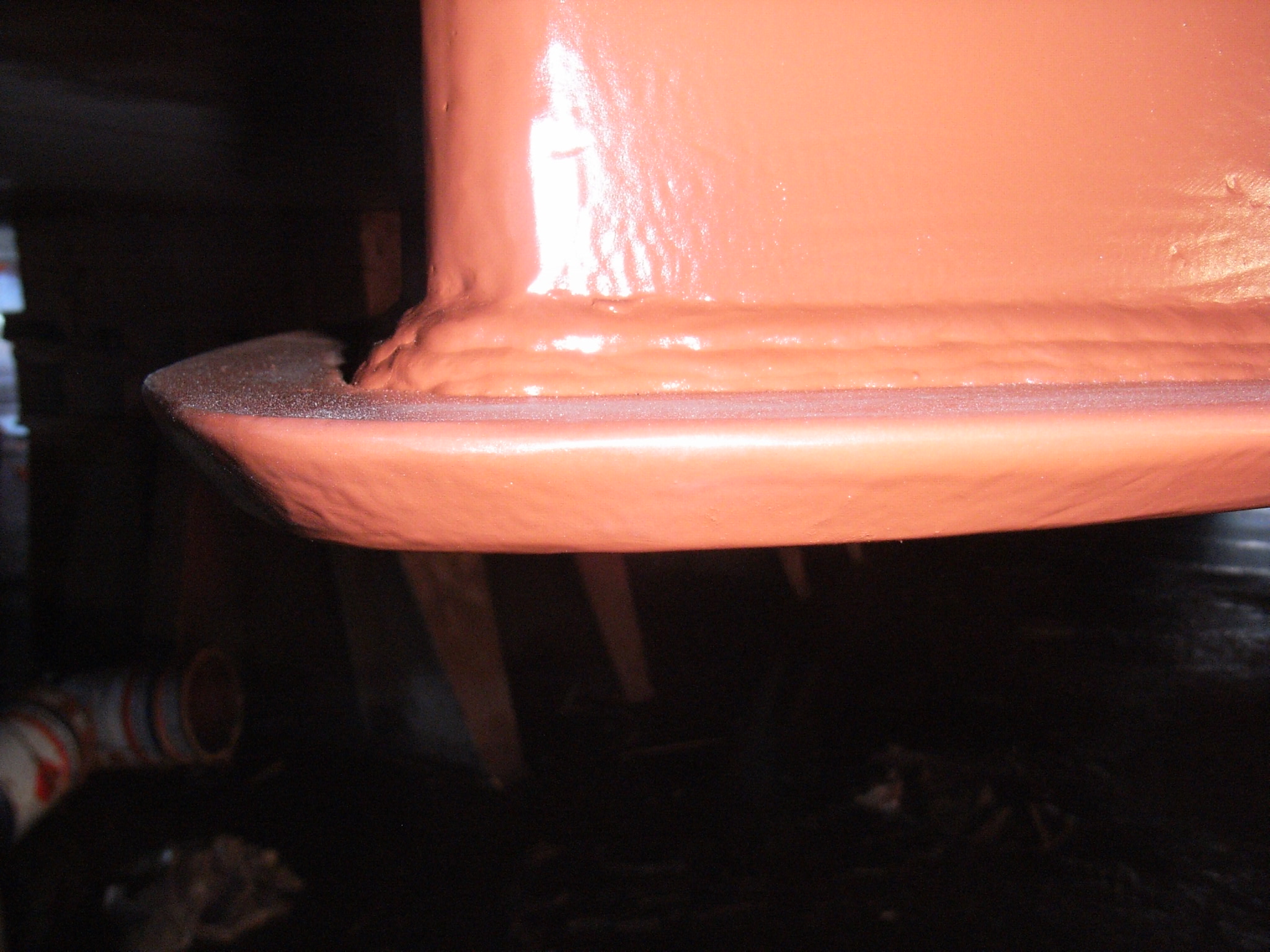
the surface illuminated bubble clouds from the side. In the figure below showing the bubble
fairing from the side, one can see the bubble cloud approaching
from the right. The fairing is 21
cm high indicating that this particular bubble cloud is roughly
30 cm deep. This video was obtained
when the winds and sea state were relatively mild.
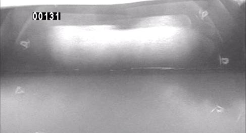
When the conditions
are much rougher, the camera’s vision is often obscured by the
bubbles next to the lens so our ideas about what is happening
may be biased. The second figure
below was taken looking forward at a location closer to the
centerline of the ship. The grey
clouds visible below the hull are the bubble clouds approaching
the camera. A few frames later the
camera is obscured due to the bubbles hitting the lens. While the bubble clouds are
undoubtedly produced in the turbulent bow wave as the ship
pitches up and down, the shape of the clouds seem quite steady
for the two or three seconds that they show up in the videos. It is also clear that the larger
bubble clouds are produced by the pitching of the ship as they
come at the camera at fairing regular intervals.
 |
 |
| Camera view looking at the
fairing |
Camera view looking forward |
Clicking on the following links will bring you the most illustrative videos for the first four deployments: #1, #2, #3, and #4. The positions of the camera for each of the videos is shown in the figure above right. In the first video the camera is upside down so up is down and left is right. Overall, the combined camera and sonar result together with the results from the first temporary bubble fairing suggested that there will be fewer bubble problems if we moved the ADCP closer to the centerline of the ship.
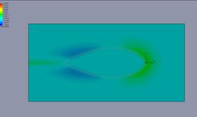
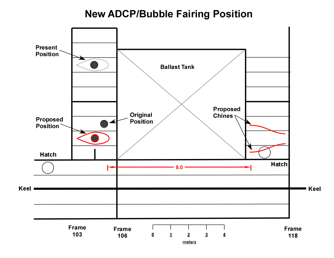
The last part of the investigation involved computational fluid dynamics simulations performed by Bob Fratantonio, a graduate student in ocean engineering at URI, using Floworks software. The questions we wanted to resolve were: 1) was there a better overall shape to the fairing than the initial one, in particular would a more pointed fairing reduce the stagnation pressure at the leading edge of the fairing, 2) would extending the lip forward to 8 cm (from the current 4 cm) help reduce the boundary layer flow under the fairing, and 3) would vertical fins or chines placed ahead of the fairing cause sufficient upwelling under the hull to bring bubble free water up against the fairing and transducer. Each of these questions was addressed in succession and then finally in combination to see how the overall system would work.
The results of altering the shape of the fairing to be more pointed does reduce the stagnation pressure at the nose of the fairing slightly and produces less of a downward deflection of particles flowing along the centerline as shown in the figure below. The figue shows path of particles released ~0.5m ahead of the fairing and 0.2m below the hull. The reduction of the stagnation pressure on either side of the centerline is more substantial with a greater effect on the flow field.
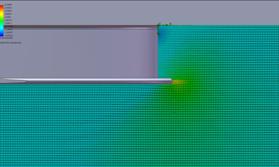
The present lip on the bubble fairing
sticks out about 2 in (5 cm) with the hope that it would reduce
the tendency for water and bubbles to flow under the fairing. This seems to work to some extent but
we were interested to see whether increasing the lip to 4 in (10
cm) would improve its performance. The
figures below show a centerline cut of the vertical velocities
using both vectors and color. It
appears that the downward vertical velocity with the extended
lip is less, but a greater effect shows up in the vertical
velocity 5 cm under the fairing. There,
the extended lip produces vortices on either side which produces
an upwelling toward the face of the fairing which seems like it
would be beneficial by bringing deeper water toward the
transducer.
 |
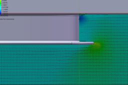 |
| Z-Velocity Side Cut Plot - 2 Inch Lip | Z-Velocity Side Cut Plot - 4 Inch Lip |
 |
 |
| Z-Velocity 5cm from Fairing Face – 2 Inch Lip | Z-Velocity 5cm from Fairing Face – 4 Inch Lip |
The last part of the investigation
involved a study of whether vertical fins oriented somewhat
across the flow could be designed in such a way that they would
cause water from farther below the ship, and hopefully with less
bubbles, to upwell toward the hull
and sweep away the bubble laden waters. A
number of configurations were tried at various distances ahead
of the fairing. The basic idea was
that a pair of fins, spreading out from the extended center of
the fairing would generate a pair of counter-rotating vortices
and upwelling along the centerline. After
some experimentation, a pair of fins 20 cm tall and about 2 m
long in the shape of a truncated hyperbolic tangent worked the
best. In the figure below chines are straight fins while rails are
fins in the shape of a hyperbolic tangent.
The top of the plot represents the bottom of the ship and
leading edge of the fairing body is at 0m.
Clearly the most effective configuration makes use of the
hyperbolic tangent rails 10 m ahead of the fairing which is able
to draw water from 0.5 m below the ship and pull it to less than
the height of the fairing itself, which is 20 cm deep.
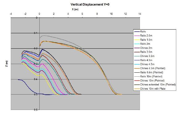 |
| Particle trajectories along the centerline for a variety of fairing shapes, fin shapes and distances ahead of the fairing. |
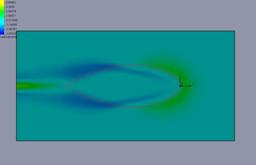
In order to extend the width of the
upwelling region, the rails extend out to 0.75 m on either side
of the centerline (the fairing itself is about half this width)
so that the upwelling covers the essentially the whole fairing
as shown in the next figure.
 |
| Plot of the vertical velocity about 25 cm below the hull of the ship. Blue is up toward the hull and yellow is downward |
The Norröna entered the drydock at the Blohm
and Voss repair yard in
 |
 |
 |
 |
 |
 |
This
web
page
is intended to be the primary method for disseminating the
ADCP data collected during the program. The data is
concatenated into yearly Codas3 data blocks which can be
accessed by clicking on the year listed below and filling out
the form. As new data is collected it will be added to the
current years' data blocks. The data can be retrieved by
specifying a date window and desired depth range and vertical
averaging. Remember that the minimum vertical binsize is 8
meters so nothing smaller than that will work. Also remember
that the upper most bins start around 20 meters so specifying
a shallower starting depth will produce NAN's even if some of
the specified bin contains usable data. The extracted data can
be returned in either flat-ASCII format or as MATLAB files.